Introducing the {metameta} R package
I'm happy to announce that I just released my first R package. Here's a quick rundown on how you can use the {metameta} package to effortlessly calculate the statistical power of published meta-analyses to better understand the evidential value of included studies.
First we'll install the package via Github and then load it. The package contains two main features:
1. Functions to calculate the statistical power of studies in a meta-analysis
2. A function to create a Firepower plot, which visualises statistical power across meta-analyses
devtools::install_github("dsquintana/metameta")
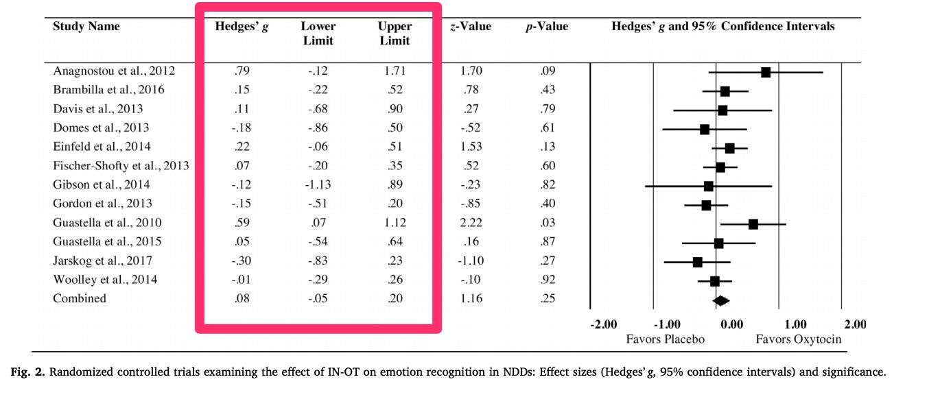
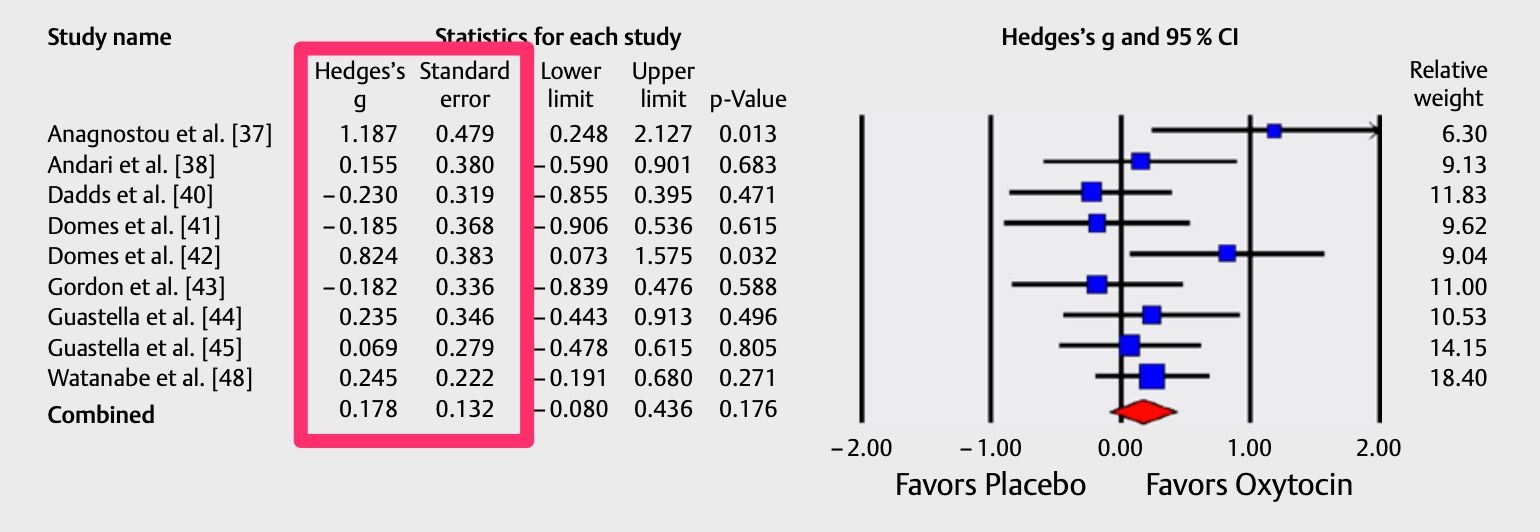
library(metameta)For first example, we're going to extract some data from this forest plot published in this meta-analysis on the impact of intranasal oxytocin on social cognition. All we need is the effect size and confidence interval data for each study included in the meta-analysis.
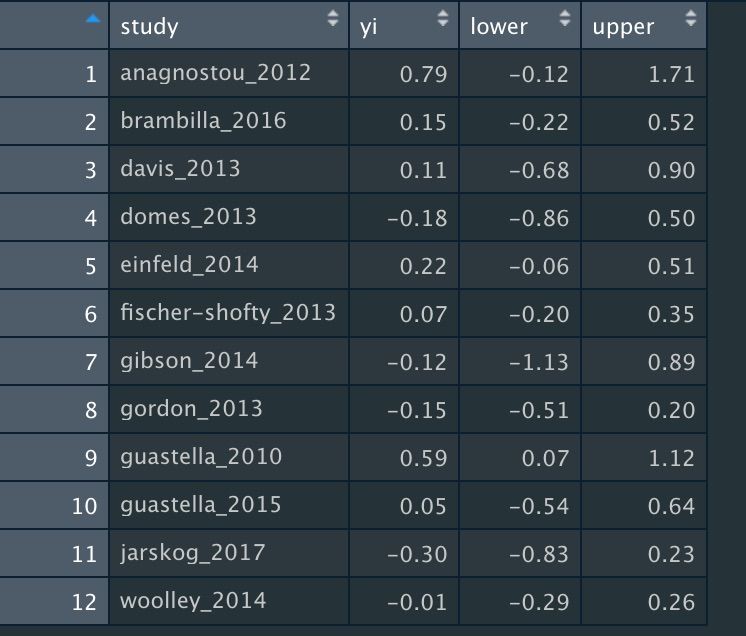
At a minimum, the dataset for analysis needs three columns, with the following labels:
1. "yi" for the effect size
2. "lower" for the lower CI bound
3. "upper" for the upper CI bound
You can also add a column for the study name, but this isn't strictly necessary.
This is what your datafile should look like:
Assuming we've named this dataset "dat_keech", we're going to use this in the mapower_ul function. This requires three arguments:
1. The data (structured as shown above)
2. The observed summary effect size estimate
3. The name of the meta-analysis (required for the other core function we'll get to soon)
power_keech <- mapower_ul(dat = dat_keech,
observed_es = 0.08,
name = "Keech et al 2017")
power_keech_dat <- power_keech$dat
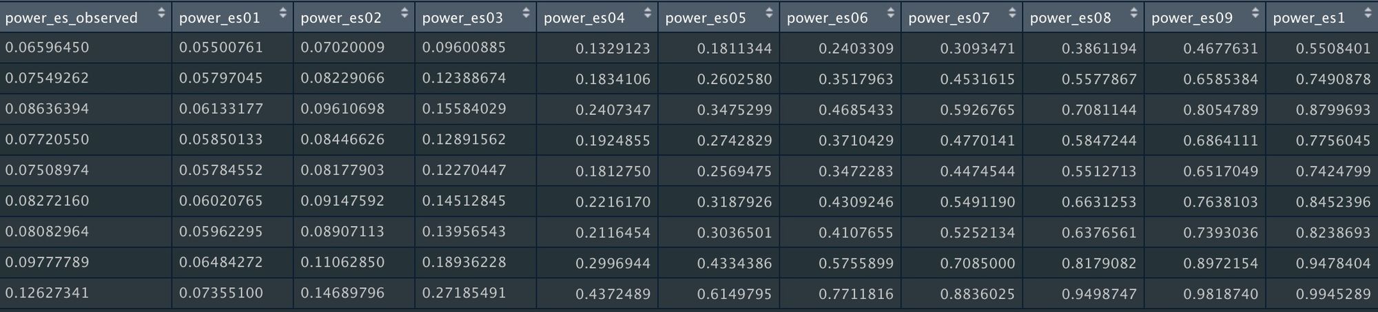
power_keech_datThis will give us statistical power for a range of possible "true" effect sizes: The reported summary effect size ("power_es_observed") and a range of effect sizes from 0.1 to 1 (in increments on 0.1).
In other words, this analysis calculates how likely it would to be observe a significant effect given a range of possible effect sizes.
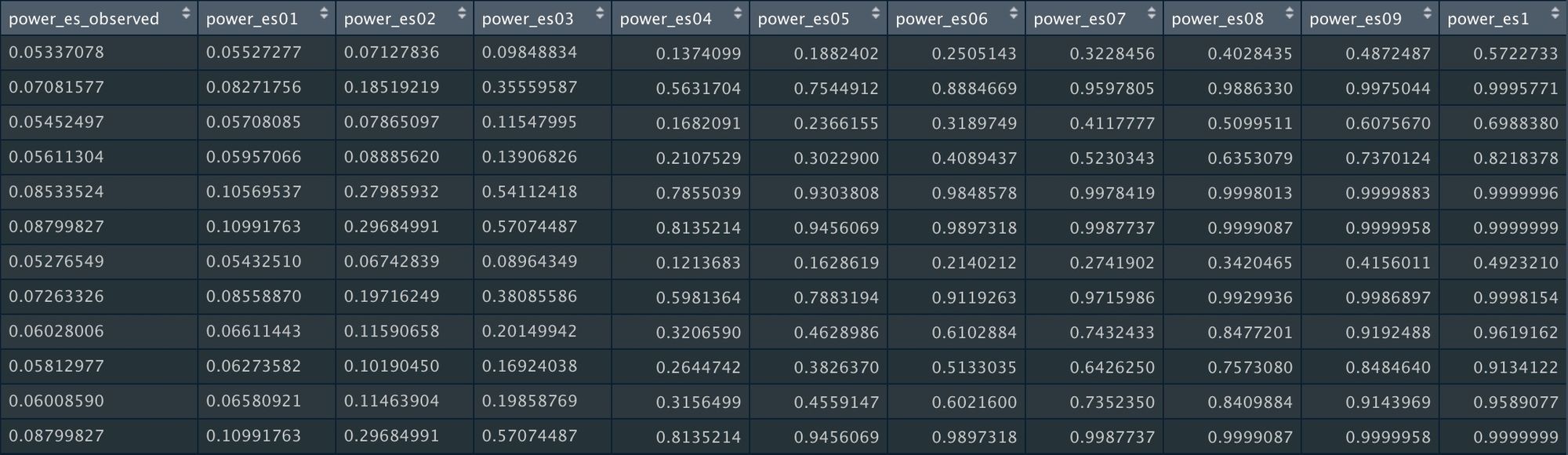
In this particular field, the average effect size is around 0.2, and that's probably inflated due to publication bias. So conservatively assuming that 0.2 is the true effect size, power ranges from 7% to 30% in these studies.
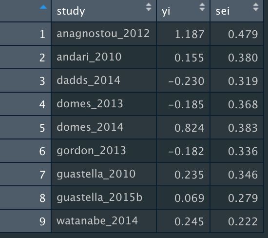
There's also a function for meta-analyses that report effect sizes and standard errors, called mapower_se. To illustrate, let's extract the data from this forest plot published in this meta-analysis.
For this function, only two columns are required:
1. "yi" for effect sizes
2. "sei" for standard errors
Assuming we've named this dataset "dat_ooi", we're going to use this in the mapower_se function. This requires three arguments, as before:
- The data
- The observed summary effect size estimate
- The name of the meta-analysis
power_ooi <- mapower_se(dat = dat_ooi,
                        observed_es = 0.178,
                        name = "ooi et al 2017")
power_ooi_dat <- power_ooi$dat
power_ooi_dat
As before, this will return the statistical power for a range of possible "true" effect sizes.
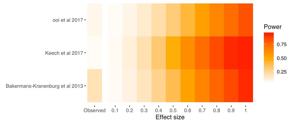
Sometimes it’s useful to calculate power for a body of meta-analyses, which might be reported in the same article or across articles. But Illustrating the power of individual studies from multiple meta-analyses can be difficult to interpret if there are lots of studies.
An alternative is to illustrate the power per meta-analysis by calculating the median power across studies. We can illustrate this with a “Firepower” plot, which we can create using the firepower function. First, we need to prepare the data.
Here, we're combining three meta-analyses into a list.
### Calcuate median power for three meta-analyses
power_ooi <- mapower_se(dat = dat_ooi,
                        observed_es = 0.178,
                        name = "ooi et al 2017")
power_med_ooi <- power_ooi$power_median_dat

keech_power <- mapower_ul(dat = dat_keech,
                          observed_es = 0.08,
                          name = "Keech et al 2017")
power_med_keech <- keech_power$power_median_dat

power_bakermans_kranenburg <-
  mapower_se(dat = dat_bakermans_kranenburg,
             observed_es = 0.32,
             name = "Bakermans-Kranenburg et al 2013")
power_med_bakermans_kranenburg <- power_bakermans_kranenburg$power_median_dat

### Create a list
list_power <- list(power_med_ooi, power_med_keech, power_med_bakermans_kranenburg)

### Run firepower function
fp <- firepower(list_power)

### Create firepower plot
fp_plot <- fp$fp_plot
fp_plot
And here's our Firepower plot

You can also extract the raw data underlying this plot:
library(tibble)
fpdata <- fp_plot$data
fpdata <- as_tibble(fpdata)
fpdata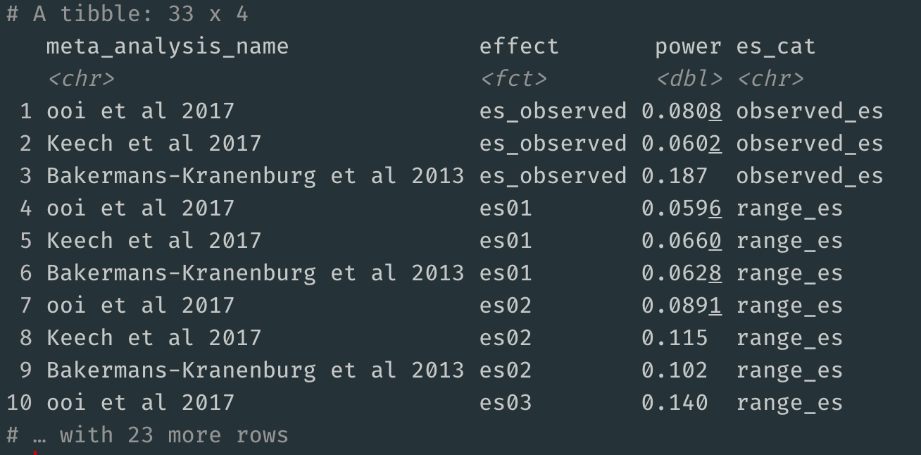
Try out this package for yourself either using the three example datasets or your own data. If you find any bugs or have feature requests, please file an issue on the package's GitHub page.