How to visualise the power of each effect in a meta-analysis

Garbage in, garbage out is a common criticism of meta-analysis. While I'm generally a fan of meta-analysis, I think this is a very fair critique.

One approach to determine the evidential value of studies included in a meta-analysis is to determine the statistical power of the reported tests that were used. Tests with low statistical power have a low probability of finding a statistically significant effect, if there's a true effect to be found. This also means that tests with low statistical power are less likely to replicate. Consequently, a meta-analysis that contains studies with low power is likely to comprise results that won't replicate and a summary effect size estimate that is inflated.

You can calculate statistical power one-by-one for each effect size, but this is time consuming. However, it's possible to calculate statistical power using the information that has already been extracted for a meta-analysis, namely, a set of effect sizes and their variances.

To demonstrate this, I'm going to use the sunset_viz function from the metaviz R package. This function creates a sunset funnel plot, which is funnel plot variant that visualises the statistial power of each test included in the meta-analysis.

This function is relatively straightforward, however, you will need to specify the "true" population effect size. There are a few approaches you can take to specify this.

1. Use the summary effect size from the meta-analysis

This is the most straightforward approach, and the default in this function, but this effect size is likely to be inflated due to publication bias.

2. Use a publication-bias adjusted effect size

There a various tools, like p-uniform, that can be used to calculate a publication bias-adjusted effect size. However, these tool has some limitations. Namely, this is should only be used for meta-analyses with low heterogeneity, and it can't be used for multilevel meta-analysis (e.g., meta-analyses that account for multiple effect sizes from individual studies).

3. Determine the smallest effect size of interest

The smallest effect size if interest (SESOI) is the smallest effect size you care about for the research question at hand. For example, if for your research question an effect size lower than d = 0.1 is essentially meaningless or has no practical value, then d = 0.1 is your SESOI. If your test is sensitive enough to to detect the smallest effect size of interest, then it's able to detect larger effects as well.

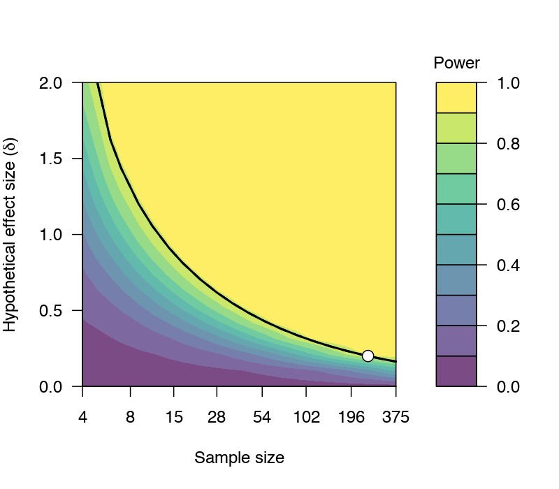
For a quick demonstration, consider this plot below, which was created by the 'jpower' module in JAMOVI. Let's say our SESOI is 0.1 and we have 250 participants for a paired samples t-test. This design can detect effect sizes of 0.2 with a probability of at least 0.88 (i.e., 88% power) when α=0.05 (two-tailed). If the "true" effect size is higher than 0.2, then the probability of detecting these effect sizes are higher than 88%.

Now, to demonstrate this tool, let's use an example correlational dataset that I've used in previous demonstrations to perform a conventional meta-analysis.

library(metafor) #Load metafor
library(metaviz) #Load metaviz
library(puniform) #Load puniform 

dat <- get(data(dat.molloy2014)) # Extract data

dat <- escalc(measure="ZCOR", 
		ri=ri, ni=ni, 
        data=dat) #Calculate effect sizes
        
res <- rma.uni(yi, vi, data=dat) 

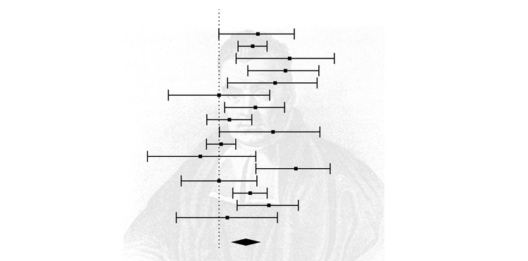
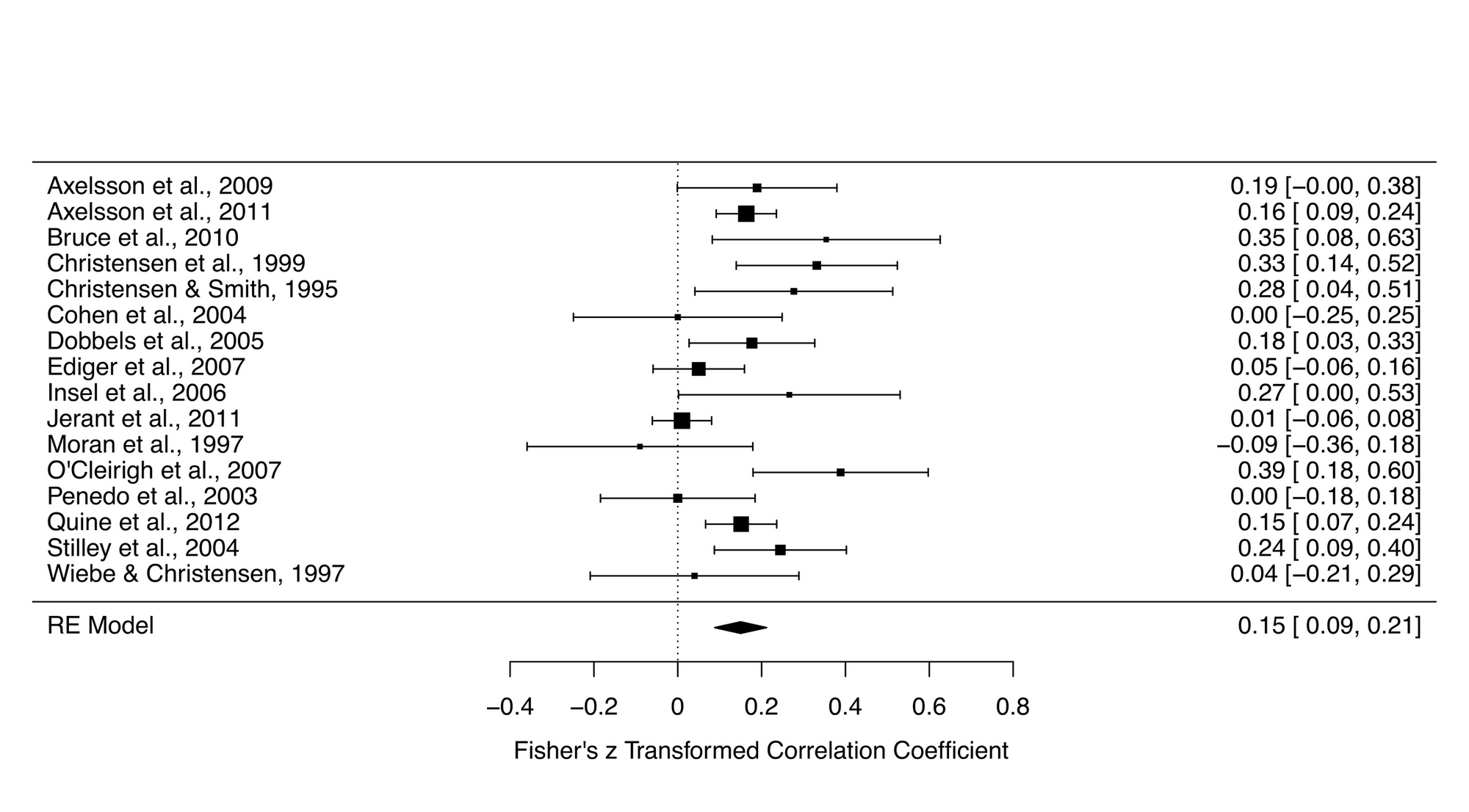
forest_plot <- forest(res)
forest_plot 

Here are the results of this meta-analysis.

Let's also make a funnel plot, which illustrates the potential for small-study bias by plotting each effect size against its standard error, centred on the estimated summary effect size.

funnel_plot <- funnel(res)
funnel_plot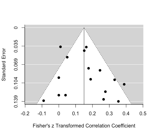

We can improve this plot by adding 'significance' contours and centring the funnel on zero.

funnel_contour <- funnel(res, level=c(90, 95, 99), 
                  shade=c("white", "orange", "red"), 
                  refline=0, legend="topleft")
funnel_contour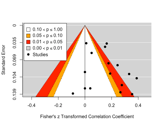

This plot show us that a few studies are lying in the 'significance' contours. While eyeballing this plot doesn't elicit too much concern for publication bias, this would still be a subjective conclusion.

To get a more objective understanding of how much publication bias is influencing the summary effect size estimate, we can adjust for publication bias using the puniform package.

puni_star(yi = dat$yi, vi = dat$vi, 
                      side = "right")

This analysis suggests that the publication bias adjusted estimate is 0.11, which is a little lower than the original estimate of 0.15.

So now we have two (out of our three) options for determining the "true" effect size. For the third option, let's assume that the smallest correlation coefficient we care about is 0.05.

We're now ready to calculate power and create a sunset plot. Let's begin by using the original effect size estimate. By default, this function uses the original effect size estimate so you don't need to specify it.

viz_sunset(res, 
           contours = TRUE,
           power_contours =  "continuous")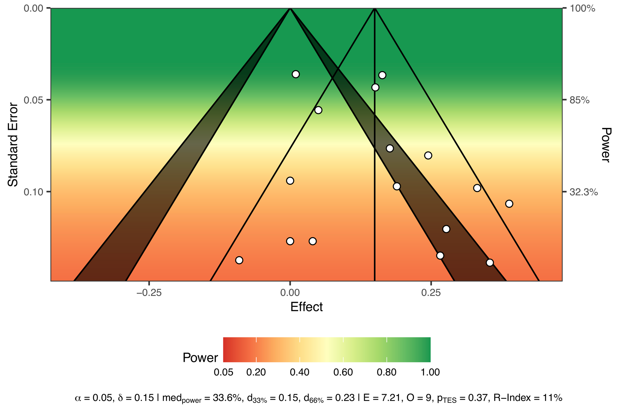

Let's walk through this plot.

Power is visualized by colour, with red used for "danger", as in, "these tests are very underpowered". The description at the bottom also displays the following:

• The alpha (0.05)
• The true effect size (0.15)
• The median power of all the tests (33.6%)
• The true effect size needed for achieving 33% (0.15) and 66% (0.23) of median power
• Results from a test of excess significance (i.e., given the data we would expect 7.21 statistically significant studies and we observed 9, yielding a p-value of 0.37)
• An R-Index measure of 11%, suggesting that these studies have a low probablility of replicating

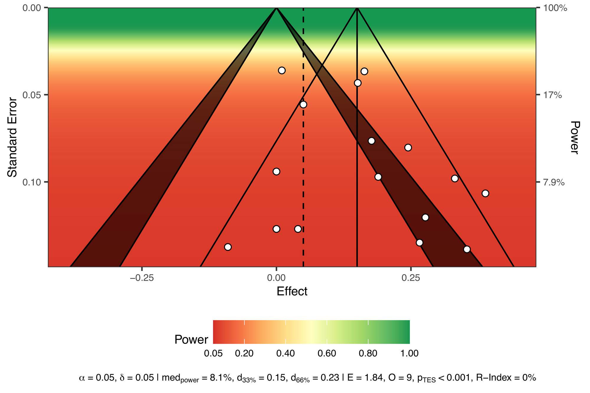
To use our minimally interesting effect for the true effect size, we just need  to tweak the code a little.

viz_sunset(res, 
           contours = TRUE,
           true_effect = 0.05,
           power_contours =  "continuous")

All tests reported from these studies are underpowered to detect this minimally interesting effect.

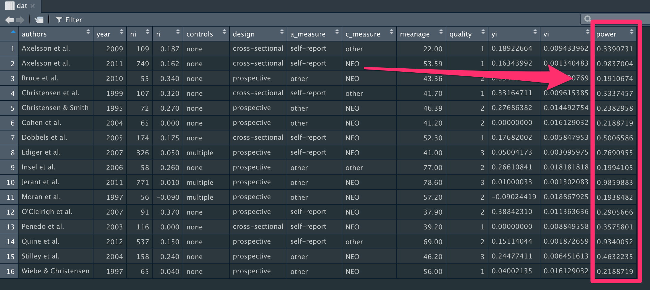
Finally, if you are interesting in extracting the exact power values, I have put together a small custom function.

s_power <- function(se, true_effect, sig_level) {
  
  (1 - stats::pnorm(stats::qnorm(1 - sig_level/2) * 
                      se, abs(true_effect), se)) + 
    stats::pnorm(stats::qnorm(sig_level/2) * 
                   se, abs(true_effect), se)
}

Let's use this function to add power calculations to each study using a true effect size of 0.15. We also need to specify the standard error for each effect, and significance level. Here, we're using data from the funnel plot we made earlier to extract the standard error information.

dat$power <- s_power(se = funnel_plot$y, 
               true_effect = 0.15, 
               sig_level = 0.05)

Now we have the precise power estimates for each effect size at the end of our dataset.

Here's the full script, if you'd like to run this all in one go.

library(metafor) #Load metafor
library(metaviz) #Load metaviz
library(puniform) #Load puniform 

dat <- get(data(dat.molloy2014)) # Extract data

dat <- escalc(measure="ZCOR", 
              ri=ri, ni=ni, 
              data=dat) #Calculate effect sizes

res <- rma.uni(yi, vi, data=dat) 

forest_plot <- forest(res)
forest_plot 

funnel_plot <- funnel(res)
funnel_plot

funnel_contour <- funnel(res, level=c(90, 95, 99), 
                  shade=c("white", "orange", "red"), 
                  refline=0, legend="topleft")
funnel_contour

puni_star(yi = dat$yi, vi = dat$vi, 
                      side = "right")

viz_sunset(res, 
           contours = TRUE,
           power_contours =  "continuous")


viz_sunset(res, 
           contours = TRUE,
           true_effect = 0.05,
           power_contours =  "continuous")


s_power <- function(se, true_effect, sig_level) {
  
  (1 - stats::pnorm(stats::qnorm(1 - sig_level/2) * 
                      se, abs(true_effect), se)) + 
    stats::pnorm(stats::qnorm(sig_level/2) * 
                   se, abs(true_effect), se)
}

dat$power <- s_power(se = funnel_plot$y, 
               true_effect = 0.15, 
               sig_level = 0.05)