Oh my GOSH: Calculating all possible meta-analysis study combinations
There are several analytical decisions that need to made when performing a meta-analysis. These decisions are not trivial, as they can influence meta-analysis outcomes and conclusions.
One of these decisions is deciding which studies to include in the meta-analysis. A single study, or group of studies, can have a disproportionate influence on the summary effect size.
Let's fire up up R and have a closer look. Here, I'm going to load up the metafor package and use one its built-in meta-analysis datasets. This meta-analysis dataset from Molloy and colleagues explores the relationship between conscientiousness and medication adherence.
Here's a basic meta-analysis, which extracts the data, calculates an effect size measure and effect size variance, and creates a forest plot for visualisation.
library(metafor) #Load metafor
dat <- get(data(dat.molloy2014)) # Extract data
dat <- escalc(measure="ZCOR",
ri=ri, ni=ni,
data=dat) #Calculate effect sizes
res <- rma.uni(yi, vi, data=dat)
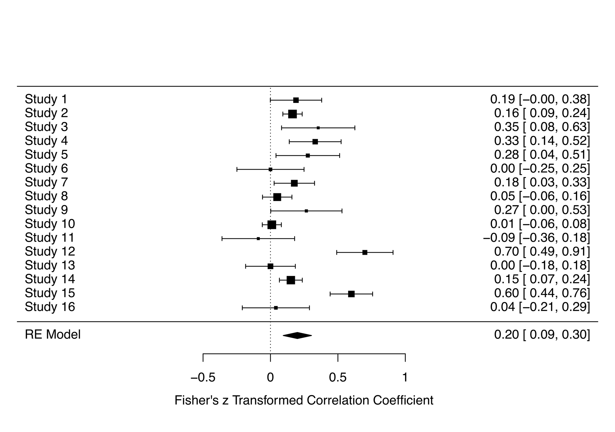
forest_plot <- forest(res)Let's look at the forest plot that was generated from this script. The summary effect size was 0.15, and this was statistically significant, suggesting a modest relationship between conscientiousness and medication adherence.
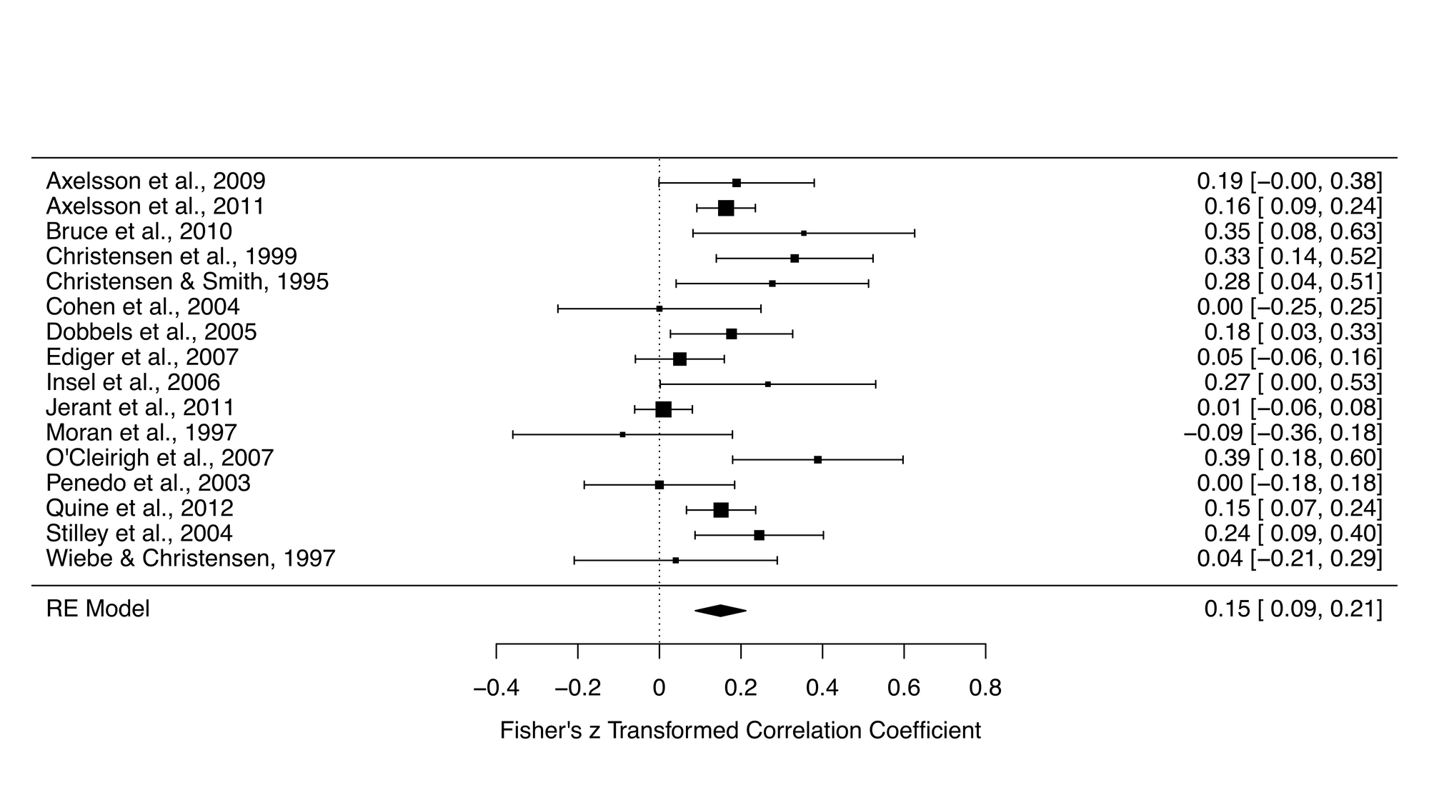
To demonstrate the robustness of the result, it's good practice to perform a leave-one-out analysis. Like the name suggests, this analysis performs a series of meta-analyses leaving one of the studies out. So if you had 15 studies in your meta-analysis, you would have 15 meta-analyses.
Here is the script to run this:
l_one <- leave1out(res)And here are the results:
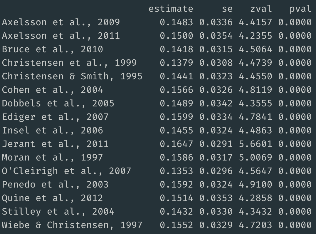
The summary effect sizes for meta-analyses that removed a single study ranged from 0.14 to 0.16. Thus, removing a single study did not have much influence on the primary summary effect size, which as 0.15.
This analysis is quite informative, but perhaps there's a distinct subgroup of studies influencing the result, rather than a single study.
So let's what's called a combinatorial meta-analysis, which performs a series of meta-analyses based on all possible combinations of studies.
The number of analyses to be conducted can be calculated using the formula 2^k - 1, with k representing the number of studies. So for a meta-analysis with 16 studies, you will perform 65535 meta-analyses, that is 2^16 - 1.
To visualise this enormous number of summary effect size estimates, we'll put together a Graphical Display of Study Heterogeneity (GOSH) plot, using the following script, but before running the script, I should warn you that this could take some time to create 65535 models (it took about 10 minutes on my 2015 MacBook Pro).
gp <- gosh(res)
g_plot <- plot(gp, breaks = 100)
g_plotHere's a visualisation of the summary effects of 65535 models (horizontal axis), plotted against the model's heterogeneity (vertical axis).
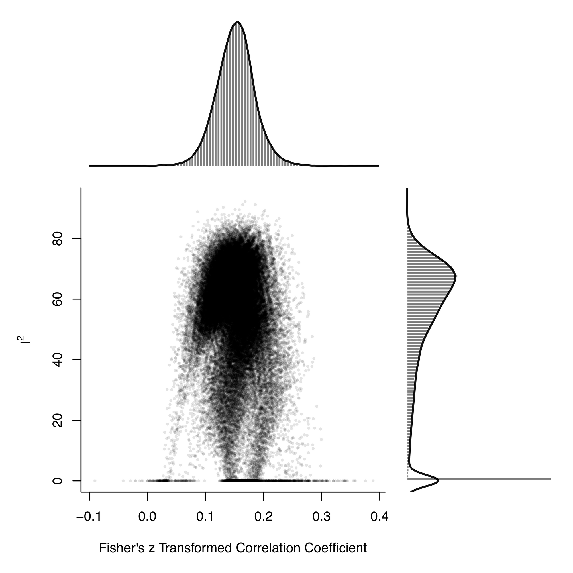
By extracting the list of effect sizes, it's straightforward to calculate the mean effect size, which is 0.15.
mgosh <- gp$res

mean_est <- mean(mgosh$estimate, na.rm = TRUE)
The effect sizes range from about 0.05 to 0.25, demonstrating how the choice of included studies influences the summary effect size estimate.
Now let's see what happens when we add in some artificial outliers, using this script:
dat_mo <- get(data(dat.molloy2014))

dat_mo <- escalc(measure="ZCOR",
                ri=ri, ni=ni, data=dat_m)

dat_mo[12,11] = 0.7
dat_mo[15,11] = 0.6

res_mo <- rma.uni(yi, vi, data=dat_mo)

forest(res_mo)
You can see the introduced outliers in the forest plot (studies 12 and 15)
Now let's run the combinatorial meta-analysis and create a GOSH plot:
gp_mo <- gosh(res_mo)

plot(gp_mo, breaks = 100)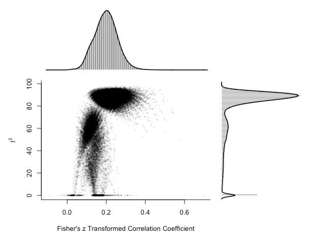
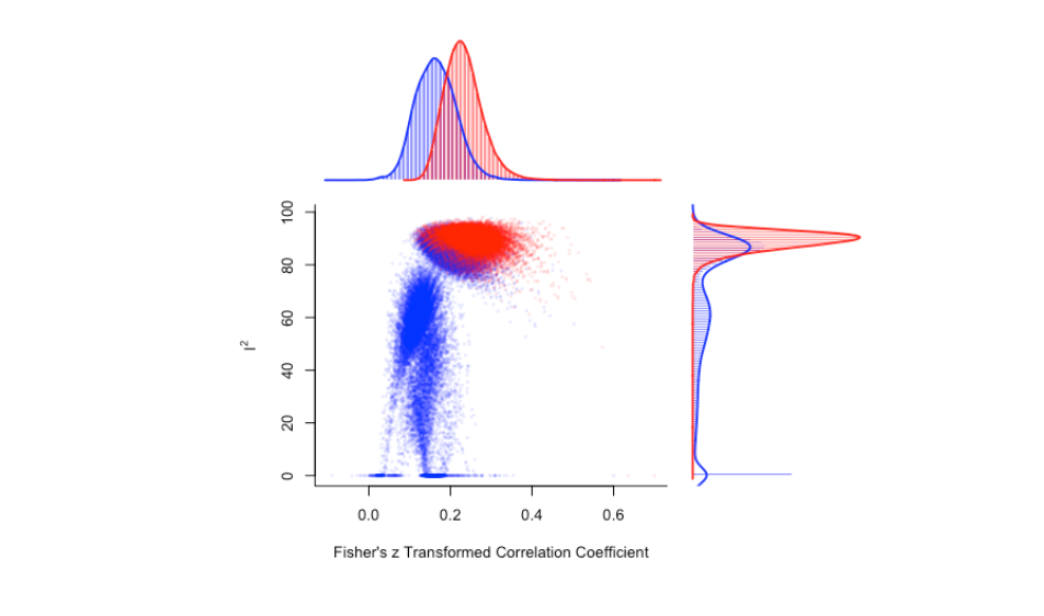
There is a clear cluster of large effect sizes with high heterogeneity in the top right of the plot. We can specifically highlight the meta-analysis models that included the potential outlier studies:
plot(gp_mo, out=12, breaks = 100)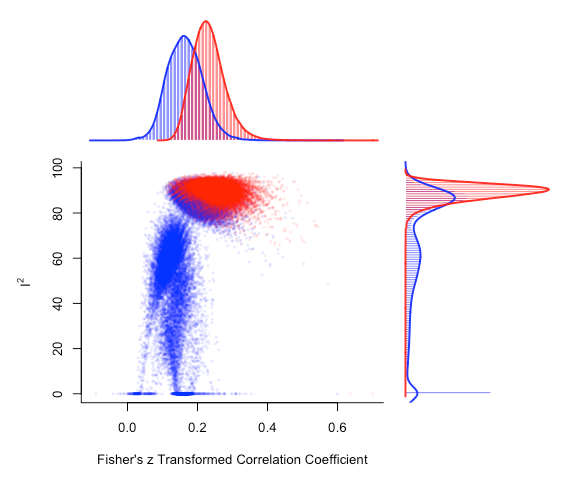
There's a noticeable shift in the distribution of meta-analysis model summary effect size estimates that include study 12.
Ultimately, combinatorial meta-analysis paired with GOSH plots demonstrate how your analysis choices influence your meta-analysis outcomes and conclusions.