How to perform a Bayesian meta-analysis
Meta-analyses conventionally adopt a frequentist approach, in which a p-value is used to make a binary decision regarding the presence of an effect. While correctly used p-values can be useful, using a Bayesian framework can provide a number of benefits for the meta-analyst. However, Bayesian meta-analysis is uncommon, probably due to a historical lack of accessible software options for performing these tests. So in this post I'm going to outline the benefits of Bayesian meta-analysis and a step-by-step guide (with code) on to perform one using the relatively new "RoBMA" R package.
I've previously outlined the benefits of using a Bayesian framework for hypothesis testing in a 2018 paper, but there are two benefits that are particularly interesting for meta-analysis, which are worth covering before diving into the code.
First, Bayes factors are an intuitive metric for describing and understanding the relative evidence for two models, typically an alternative model vs. a null model. So using this approach, one could say that there's 12 times more evidence for an alternative model compared to a null model, for instance. Of course, frequentist meta-analysis can be reported with effect sizes, but interpreting effect sizes can be difficult, as Cohen's benchmarks of small/medium/large effects are not universal across research fields.
Second, non-significant p-values carry very little information, as these values can either suggest the absence of evidence or evidence of absence, regardless of the size of your p-value. As alluded to above, with Bayes factors you can also assess the relative evidence for a null model compared to an alternative model (unlike null hypothesis testing in which you can only reject a null hypothesis). Along with estimating the relative evidence for meta-analytic models, Bayes factors can also be used to estimate the relative evidence for publication bias. Frequentist approaches for publication suffer this same limitation, in that a non-significant test for publication bias can either suggest the absence of evidence or evidence of absence.
To illustrate the differences between a frequentist and Bayesian meta-analysis, I'm going to use an example that I've used for a previous tutorial paper for a frequentist meta-analysis. This dataset contains 17 studies that report the correlation between medication adherence and a measure of conscientiousness.
Let's run a frequentist analysis and construct a forest plot to visualise the result using the following script:
library(metafor) #load the metafor package
dat <- dat.molloy2014 # Extract the dataset
dat <- escalc(measure="ZCOR",
ri=ri, ni=ni,
data=dat.molloy2014,
slab=paste(authors, year, sep=", "))
res <- rma(yi, vi, data=dat) # Perform meta-analysis
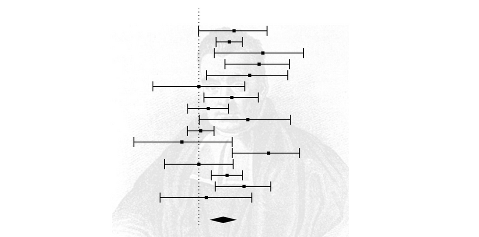
res # print resultsHere are the results, followed by a forest plot:
Random-Effects Model (k = 16; tau^2 estimator: REML)

tau^2 (estimated amount of total heterogeneity): 0.0081 (SE = 0.0055)
tau (square root of estimated tau^2 value):      0.0901
I^2 (total heterogeneity / total variability):   61.73%
H^2 (total variability / sampling variability):  2.61

Test for Heterogeneity:
Q(df = 15) = 38.1595, p-val = 0.0009

Model Results:

estimate      se    zval    pval   ci.lb   ci.ub
  0.1499  0.0316  4.7501  <.0001  0.0881  0.2118  ***

---
Signif. codes:  0 ‘***’ 0.001 ‘**’ 0.01 ‘*’ 0.05 ‘.’ 0.1 ‘ ’ 1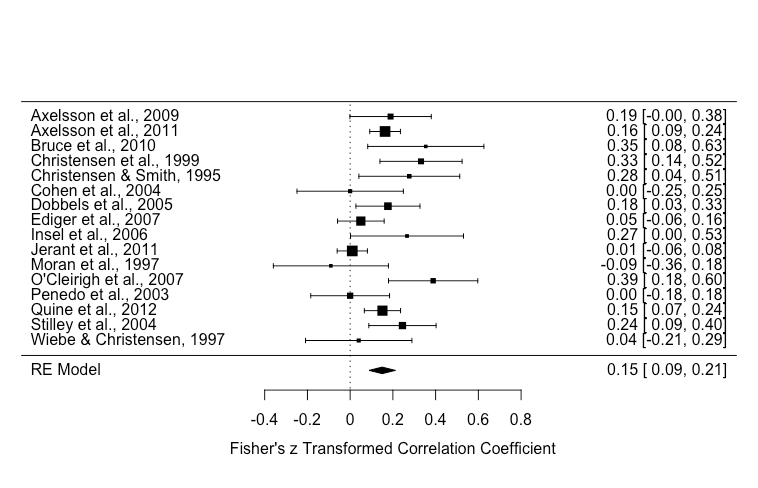
Of note, there was significant heterogeneity [Q(df = 15) = 38.1595, p-value = 0.0009] and the effect size estimate was 0.15 (p < .001).
Conventionally, a meta-analyst would construct a funnel plot and perform Egger's regression test to assess publication bias via funnel plot asymmetry. But as I've outlined before, funnel plot asymmetry can only assess small study bias which can include publication bias, but also other factors (e.g., study quality).
funnel(res)

regtest(res)

# regtest results #

Regression Test for Funnel Plot Asymmetry

Model:     mixed-effects meta-regression model
Predictor: standard error

Test for Funnel Plot Asymmetry: z = 1.0216, p = 0.3070
Limit Estimate (as sei -> 0):   b = 0.0790 (CI: -0.0686, 0.2266)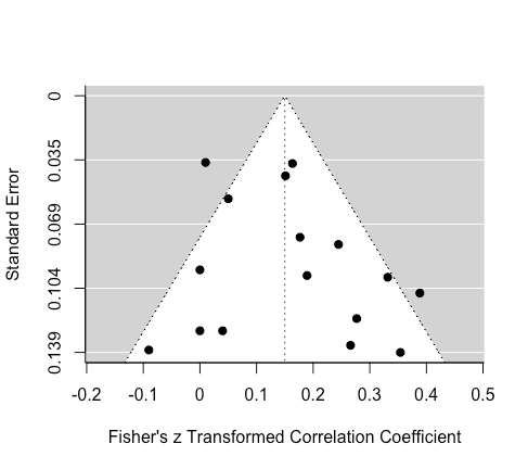
Eyeballing the funnel plot suggests that the distribution of effects is fairly symmetrical. Egger's regression test was non-significant, which suggest either that there is either no asymmetry or the data were not sensitive enough.
Next, let's use an approach that that has been designed to specifically assess publication bias: weight-function models. In short, weight-function models provide a greater weight to studies that were less likely to have been published, based on their associated p value, for the estimation of a summary effect size. For example, it is a fair assumption that a study with a p value of 0.001 is more likely to be published than a study with a p value of 0.45. Other methods for publication bias detection and correction have been proposed, but weight-function models seem to perform the best across a range of situations (e.g., high heterogeneity).
It's worth emphasizing two limitations with selection models: 1) These models assume that the chosen selection model is an good approximation for the underlying selection process (i.e., that the chances of publication depend on the p value). But despite this limitation, weight-function models at least make the selection process is explicit (whereas this the selection process is implicit in other methods, which means they can't be evaluated). 2) Selection-models (like other publication bias methods) are a type of sensitivity analysis, which means that the publication bias model is an estimate that isn't based on real numbers, but a set of assumptions for the how the chances of publication depends on the p value.
There are various approaches for selection models (e.g., a beta model, a power model), but here we will use the Vevea and Hedges (1995) step function approach, which is implemented in the weightr package:
library(weightr)

weightfunct(dat$yi, dat$vi)

Unadjusted Model (k = 16):

tau^2 (estimated amount of total heterogeneity): 0.0070 (SE = 0.0051)
tau (square root of estimated tau^2 value):  0.0834

Test for Heterogeneity:
Q(df = 15) = 38.1595, p-val = 0.001436053

Model Results:

          estimate std.error z-stat      p-val   ci.lb  ci.ub
Intercept   0.1486   0.03073  4.835 1.3288e-06 0.08837 0.2088

Adjusted Model (k = 16):

tau^2 (estimated amount of total heterogeneity): 0.0056 (SE = 0.0045)
tau (square root of estimated tau^2 value):  0.0750

Test for Heterogeneity:
Q(df = 15) = 38.1595, p-val = 0.001436053

Model Results:

              estimate std.error z-stat    p-val    ci.lb  ci.ub
Intercept      0.09153   0.04464  2.050 0.040341  0.00403 0.1790
0.025 < p < 1  0.24121   0.20122  1.199 0.230626 -0.15317 0.6356

Likelihood Ratio Test:
X^2(df = 1) = 2.98493, p-val = 0.084043
This output might be new for many people reading, so I'm going to walk through it.
The "model results" section displays the conventional results, in terms of heterogeneity and effect size estimates. Note that the results are not exactly the same as our first analysis above, this is because the weightr package converts correlations to Cohen's d effect sizes for the analysis, and then transforms these results back to correlations.
The "adjusted model" section includes results accounting for publication bias (note the results in the "intercept" row). The summary effect estimate has shrunk from 0.15 to 0.09, and it is now very close to the threshold of statistical significance. (p = 0.04). A formal comparison of these two models, which tests for publication bias, was statistically significant using a threshold of p = 0.1, which has been recommended by Renkewitz & Keiner, along with Begg & Mazumdar.
This shifted threshold highlights the arbitrary nature of p-value thresholds. Strictly using the conventional significance threshold of p = 0.05, one would conclude that there was no publication bias. However, using a significance threshold of p = 0.1, one conclude that there's indeed publication bias.
As mentioned above, but worth repeating, Bayes factors are values that represent the relative evidence for two competing models, without requiring a strict cutoff. This means that we can do away with the need for making a binary decision when it comes to evaluating the presence of publication bias.
So let's now jump in and perform Bayesian hypothesis tests using the RoBMA R package. This package generates three families of models, across 12 models, then averages their performance. These models vary on whether they're fixed or random effects models (i.e., assuming heterogeneity), a null or alternative hypothesis models, or whether models include the presence of publication bias or not. In terms of publication bias models, separate models also use a two-step approach (significant or non-significant) or a three-step approach (significant, marginally significant, or non-significant). For more information, see Maier and colleagues.
Before running this analysis, just keep in mind that this can take some time, depending on the speed of your computer. It took my five-year-old MacBook Pro just over five minutes to complete these analyses, for reference.
fit <- RoBMA(r = dat$ri,
             n = dat$ni,
             study_names = dat$authors,
             seed = 2333)

summary(fit)

## OUTPUT ###

Call:
RoBMA(r = dat$ri, n = dat$ni, study_names = dat$authors, seed = 2333)

Robust Bayesian Meta-Analysis
              Models Prior prob. Post. prob. Incl. BF
Effect          6/12       0.500       0.992  119.310
Heterogeneity   6/12       0.500       0.963   25.726
Pub. bias       8/12       0.500       0.544    1.194

Model-averaged estimates
                 Mean Median 0.025 0.975
mu              0.129  0.129 0.057 0.202
tau             0.163  0.158 0.000 0.320
omega[0,0.05]   1.000  1.000 1.000 1.000
omega[0.05,0.1] 0.814  0.956 0.252 1.000
omega[0.1,1]    0.718  0.848 0.153 1.000
(Tau is on Cohen's d scale.)
(Estimated omegas correspond to two-sided p-values)
Let's go through these results, first addressing the "Robust Bayesian meta-analysis" section. The "Effect" row includes a Bayes Factor ("Incl. BF") of 119, which indicates that there is 119 times more evidence for an effect model relative to a null model. The "Heterogeneity" row indicates that there is 26 times more evidence for a heterogeneity model than a model without heterogeneity. Finally, the "Pub. bias" row indicates that there's 1.2 times more evidence for a publication model than a model without publication bias, which is very small evidence.
The "Model-averaged estimates" section contains an estimate of the summary effect size (mu), which was 0.13. Keep in mind that this is the values that is averaged across all models, including publication bias models, so this is a publication bias adjusted value.
Let's compare this model-averaged estimate against the a model that parallels the conventional frequentist approach: A model that assumes an effect with heterogeneity and no publication bias (i.e., a random-effects meta-analysis). This is model #10 in our analysis, and information for this model can be found by entering this command: summary(fit, type = "individual"). This command will list information from all 12 models (output not shown here for the sake of space). For model #10, the mean estimate was 0.15, which mirrors our conventional frequentist analysis above.
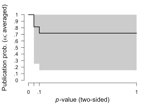
The "Model-averaged estimates" section also provides interesting information regarding the relative probability of publication of results of significant (the omega[0,0.05] row), marginally significant (the omega[0.05,0.1] row), and non-significant (the omega[0.1,1] row) results. This analysis suggested there was 100% probability that significant results (p < 0.05) were published, which is a consequence of how the model was set up, a 81.4% probability that marginally signficant results (.05 < p < .10) were published (relative to significant studies), and 71.8% chance that non-significant results (p > 0.1) were published (relative to significant studies).
We can also plot these results using this command: plot(fit, parameter = "omega")
It's also important to check the diagnostics of these 12 models to identify any issues. Rhat convergence and the effect sampling size (ESS) provide a summary of Markov chain Monte Carlo (MCMC) convergence for the appropriateness of drawing inferences. It's recommended that Rhat convergence values should be under 1.05 and that the effect sampling size (ESS) is sufficiently large. There's no clear rule-of-thumb for what constitutes a "large" ESS, but even an ESS of a few hundred is fine if you're only interested in the posterior means. We can easily generate a summary including diagnostics with this code:
summary(fit, type = "models", diagnostics = TRUE)

# OUTPUT WITH SOME INFO OMITTED FOR SPACE #

Models diagnostics overview
                  Prior mu                 Prior tau
1                 Spike(0)                  Spike(0)
2                 Spike(0)                  Spike(0)
3                 Spike(0)                  Spike(0)
4                 Spike(0) InvGamma(1, 0.15)[0, Inf]
5                 Spike(0) InvGamma(1, 0.15)[0, Inf]
6                 Spike(0) InvGamma(1, 0.15)[0, Inf]
7  Normal(0, 1)[-Inf, Inf]                  Spike(0)
8  Normal(0, 1)[-Inf, Inf]                  Spike(0)
9  Normal(0, 1)[-Inf, Inf]                  Spike(0)
10 Normal(0, 1)[-Inf, Inf] InvGamma(1, 0.15)[0, Inf]
11 Normal(0, 1)[-Inf, Inf] InvGamma(1, 0.15)[0, Inf]
12 Normal(0, 1)[-Inf, Inf] InvGamma(1, 0.15)[0, Inf]
                         Prior omega max(MCMC error) min(ESS) max(Rhat)
1                           Spike(1)              NA       NA        NA
2          Two-sided((0.05), (1, 1))           0.000     7776     1.000
3  Two-sided((0.1, 0.05), (1, 1, 1))           0.002     8239     1.001
4                           Spike(1)           0.001    18675     1.000
5          Two-sided((0.05), (1, 1))           0.003     7924     1.001
6  Two-sided((0.1, 0.05), (1, 1, 1))           0.002     7786     1.000
7                           Spike(1)           0.000    30050     1.000
8          Two-sided((0.05), (1, 1))           0.002     9407     1.001
9  Two-sided((0.1, 0.05), (1, 1, 1))           0.002     8700     1.000
10                          Spike(1)           0.001    12525     1.000
11         Two-sided((0.05), (1, 1))           0.002     9540     1.000
12 Two-sided((0.1, 0.05), (1, 1, 1))           0.002     8049     1.001
For all of our models, the largest Rhat convergence values [the max(Rhat) column] column was 1.001 and the smallest ESS [min(ESS) column] was 7776, so we can be confident of good MCMC convergence, and be on our way. If Rhat convergence values are over 1.05 or ESS values are below a few hundred, then you can try re-running your analysis with an increased number of sampling iterations and burnin. Of course, this will take longer to compute.
Keep in mind that these analyses are using a series of default prior distributions, which are designed to represent typical effects in the psychological sciences. For details on adjusting the your prior distributions, see Maier and colleagues.
In summary, our analysis revealed only very small evidence in favour of presence publication bias. Consequently, there is was only a very modest reduction in the size of the summary effect estimate after adjusting for publication bias.
So what have we learned here? First, common approaches for assessing publication bias don't actually assess publication bias. A weighted-model approach can be used as a sensitivity measure to assess the potential presence of publication bias in meta-analysis, but this using this approach via a frequentist framework has some limitations (e.g., a non-significant result is not terribly informative). Second, a model-averaged Bayesian meta-analysis can assess the relative evidence for publication bias and provide a publication bias-adjusted estimate. This meta-analysis is relatively straightforward to perform via the RoBMA R package.